Results

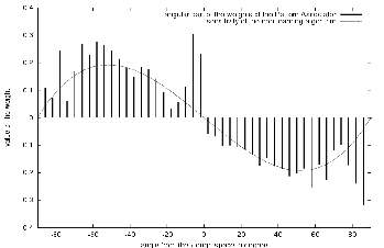
We expected that the weights of the Pattern Associator would match the perception function that we designed or at least equivalent weights which produces the same output for each inputs. Figure 3.10 shows the weights corresponding to angles in the Hough space that were learned by the Pattern Associator in this experiment.

Figure 3.10: Weights learned by the Pattern Associator. The weights match the perception function of figure 3.9 except for angles near $0^\circ$ and $90^\circ$. The detected lines for these angles correspond to the lights of the corridor.

The weights almost match the perception function. The difference comes from horizontal and vertical detected lines. These lines correspond to the lights in the corridor that are strongly detected by the edge detector because the lights saturate the pixels of the camera.

We can see that the Pattern Associator used an additional landmark to estimate the steering angle. This brings robustness to the algorithm. Indeed, if a person hides the edges of the ceiling, the Pattern Associator can still estimate a correct angle using the lights as landmarks. Of course, the robot will turn less quickly, but it will at least turn in the right direction. If the lights are hidden then the edges of the ceiling can still be used as landmarks.

The fact that the edges of the ceiling and the edges of the lights are usually distinct and far from each other in the image makes it harder for a single person to hide both features. So the learned relationship between images and steering angle is robust and can be used in real environments.

In order to assess the performance of this corridor following algorithm, several tests were made in different corridors. For each test, we used similar computation as in [20] and [8] to correct the odometry and then compute a correct performance measure based on the same characteristics of each trajectories. Figures 3.11(a) and 3.11(b) show an example of corrected odometry. The first point should be the same for each trajectories and the mean direction is also the same. This transformation is achieved by a combination of a translation and a rotation around the first point.

Figure 3.11: Correction of the odometry drifts. The raw values are translated and rotated to have the same starting point and the same mean direction.

This transformation allows us to compute the mean distance $\overline{d}$ between the trajectory and the mean direction. This is a measure of performance. If this measure gives a big value, then the trajectory is far away from its mean direction. That means that it is more chaotic than a trajectory which small value of the measure. Indeed in the ideal case, the robot follows the corridor in a straight line, and so the measure gives us the value zero.

Figures 3.12(a), 3.12(b) and 3.12(c) show the results of the test of this algorithm in three different corridors. With the measure of performance we have chosen, we have $\overline{d_a}=0.54\; in=1.37\; cm$, $\overline{d_b}=1.96\; in=4.98\; cm$ and $\overline{d_c}=0.66\; in=1.68\; cm$. So we can see that there is not a big difference between the trajectories and their mean directions. In practice, the robot seems to follow a straight line by going slightly on the right, then slightly on the left, then slightly on the right, and so on.

Figure 3.12: Results of corrected odometry for all the experiments. The training was done in the first corridor.

We can note that the training was done in the first corridor, so the performance of the first test is less realistic than the performance of the other. Indeed the learning stage could have caught the basic configuration of the corridor, that is the location of the doors and posters and the test could then be more successful in this corridor than the others. In fact, it is slightly the case, as we can see in the results of respective performances.

In the second corridor, we can notice that one of the trajectories ends before the end, and turns suddenly. This behaviour was caused by the safety procedure which caught a door frame with the sonars. It should not have caught this door frame because it was far enough, so it is certainly a freak sonar value as it happens sometimes. Anyway this behaviour is not a failure in the corridor following algorithm.

The algorithm used did not fail during the tests. However the robot was always correctly positioned in the corridor, looking at the end of the corridor. Some tests were done to estimate the robustness to the angle between the direction of the corridor and the original direction of the robot. The table 3.3 shows the maximum angle we can use to place the robot at the beginning if we want it to perform its task.

Table 3.3: Maximum original angles between the robot and the corridor.

	left	right
Corridor one	$-11^\circ$	$33^\circ$
Corridor two	$-11^\circ$	$33^\circ$
Corridor three	$-11^\circ$	$22^\circ$

In order to find the figures of table 3.3, the robot has been tested by increasing the original angle it did with the corridor. $11^\circ$ has been added each time, and when the robot failed, a second test was made with the same angle to be sure that the robot usually fails with this original angle formed with the direction of the corridor. So we can see that the allowed range of angles is not very wide but sufficient enough to dispose the robot without accuracy at the beginning of a test or in normal use. We could not expect a better accuracy because the program that learned the robot how to follow a corridor what already not really good for big angles.

We can also see that the robot performs better if it is oriented toward the right than towards the left at the beginning. This could seem strange because there is no differentiation between the left and the right in the algorithm. Indeed, this difference comes from the layout of the first corridor where the learning took place. There was a notice board near the start position on the left hand side. Because of this notice board, a big shadow projected on the wall prevented the robot from learning correctly how to avoid a wall when facing it. On the contrary, the right wall was correctly illuminated. So the robot could correctly learned how to avoid a right wall when facing it.