Comparison of learnings using the Matusita distance

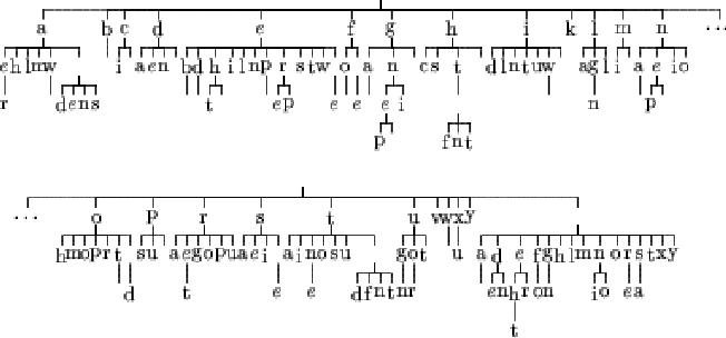
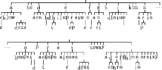
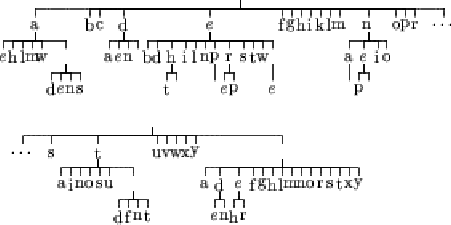
For these experiments, the VLMM has been trained on a 2144 letters long text. The training text tells the story of penguins and other animals.

Figures 6.1, 6.2, 6.3 and 6.4 represents the resulting tree for learnings done using the Matusita distance. The Lidstone estimation of probability has been used with $\lambda$ varying from 0 to 1. The case $\lambda=0$ corresponds to the maximum likelihood estimate and the case $\lambda=1$ correspond to Laplace's law of succession.

Figure 6.1: VLMM tree learned using the maximum likelihood estimation of probability and the Matusita distance. $\epsilon$ is set to 0.003 and only the probabilities that are greater than 0.003 are shown on the graph.

Figure 6.2: VLMM tree learned using the Lidstone estimation of probability with $\lambda =0.05$ and the Matusita distance. $\epsilon$ is set to 0.003 and only the probabilities that are greater than 0.003 are shown on the graph.

Figure 6.3: VLMM tree learned using the Lidstone estimation of probability with $\lambda =0.1$ and the Matusita distance. $\epsilon$ is set to 0.003 and only the probabilities that are greater than 0.003 are shown on the graph.

Figure 6.4: VLMM tree learned using the Laplace estimation of probability and the Matusita distance. $\epsilon$ is set to 0.003 and only the probabilities that are greater than 0.003 are shown on the graph.

We can see that the topology of the tree involves a lot from the case $\lambda=0$ to the case $\lambda=1$.

For the case $\lambda=1$ (figure 6.4), the depth of the tree is one. That means that the model does not take histories into account. It only models the probability of having a letter in the alphabet. We can notice that some letters like "j" or "q" are not in the tree because of their small probability in English texts, and in particular in our example text. As we have seen before, this is the problem of Laplace's law of succession because it is build on the assumption of a uniform prior.

The case $\lambda=0$ (figure 6.1), the tree seems to have learn the text in a more appropriate manner. We can find parts of some words like "peng" which comes from "penguin" (main subject of the text). We can also find small words such as "the ", "of ", "in ", "on " or "as ".

The other cases show that there is a transition between those two extremes.

This qualitative evaluation seems to be favorable to the maximum likelihood estimation. A quantitative evaluation of these trees are done later in this chapter.