Active appearance model

The aim of active appearance search is to find the parameters of the statistical appearance model that best fits it to a previously unseen image. The active appearance model search is based on the idea that the reconstruction of the image should be close to the original image. We aim to minimise the difference between the target image and the synthesis of the model.

This minimisation is done by iteratively improving a current estimate of the parameters of the model. For each step, the algorithm uses the difference between the target image and the synthesis of the model using the current estimate of the parameters. This difference is represented in a residual vector:

$${\bf r(p)}={\bf g}_s-{\bf g}_m$$ (12)

where ${\bf g}_s$ denotes the intensities in the image warped from the current shape given by the model parameters ${\bf p}$ to the mean shape and ${\bf g}_m$ denotes the intensities in the synthesis of the texture of the model. The parameters ${\bf p}$ are a concatenation of the appearance parameters ${\bf c}$, and the scale and the position of the model in the image. Figure 3.6 shows an example of the image used to compute $\vert{\bf r(p)}\vert$.

Figure 3.6: An example of difference image. The image on the left is the difference image of the target image and the model reconstruction of given parameters.

We seek to minimise the square of the norm of ${\bf r(p)}$:

$${\bf E(p)}={\bf {r(p)}}^T {\bf r(p)}$$ (13)

with respect to ${\bf p}$.

We model the residuals by assuming a local linear relationship between the parameters and the residuals:

$${\bf r}({\bf p}+\delta {\bf p}) = {\bf r}({\bf p}) + \frac{\partial {\bf r}}{\partial {\bf p }} \delta {\bf p}$$ (14)

For each step, we select $\delta {\bf p}$ which minimises ${\bf x} \mapsto {\bf E}({\bf p + x})$. We require $\frac{d {\bf E(p+x)}}{d{\bf x}} = 0$ for ${\bf x}=\delta {\bf p}$.

We have:

$${\bf E(p+x) = \left( r(p)+\frac{\partial r}{\partial p} x \right)^T \left( r(p)+\frac{\partial r}{\partial p} x \right)}$$ (15)

So:

$${\bf E(p+x) = E(p)}+2 {\bf {r(p)}^T \left(\frac{\partial r}{... ...al p} \right)^T \left(\frac{\partial r}{\partial p} \right) x}$$ (16)

This gives us the derivative of ${\bf E(p+x)}$ with respect to ${\bf x}$:

$$\frac{d {\bf E(p+x)}}{d{\bf x}}=2 {\bf {r(p)}^T \frac{\parti... ...partial r}{\partial p}\right)^T \frac{\partial r}{\partial p}}$$ (17)

By equating $\frac{d {\bf E(p+x)}}{d{\bf x}}$ to zero, we obtain:

$${\bf x^T \left(\frac{\partial r}{\partial p}\right)^T \frac{... ...al p} = - {r(p)}^T \left(\frac{\partial r}{\partial p}\right)}$$ (18)

That is:

$${\bf\left(\frac{\partial r}{\partial p}\right)^T \frac{\part... ... p} x = - {\left(\frac{\partial r}{\partial p}\right)}^T r(p)}$$ (19)

So $\delta {\bf p}$ can be computed using the formula:

$$\delta {\bf p}=- {\bf R(p) r(p)}$$ (20)

where:

$${\bf R(p)} = {\left( {\bf\frac{\partial r}{\partial p}}^T {\... ...rtial p}} \right) }^{-1} {\bf\frac{\partial r}{\partial p}}^T$$ (21)

Computing ${\bf R(p)}$ at each iteration is computationally expensive. We assume that this matrix can be considered approximatively constant, since it is computed in a normalised reference frame. So we compute it once from our training data. The equation becomes:

$$\delta {\bf p}=- {\bf R r(p)}$$ (22)

Given this model of image differences, we generate displacements ${\bf\delta p}$ around the optimal value for training images, one parameter at a time, in order to find the corresponding ${\bf r(p + \delta p)}$ by synthesis and image difference. This gives us a set of pairs $({\bf\delta p}, {\bf r(p + \delta p)})$. Those can be used to approximate the matrix ${\bf\frac{\partial r}{\partial p}}$ by averaging and combining with a normalised Gaussian kernel $w$ to smooth the result:

$$\frac{\partial r_i}{\partial p_j} = \sum_k w({\bf {\delta p}... ...) \left(r_i({\bf p + {\delta p}_{jk}} ) - r_i({\bf p}) \right)$$ (23)

where ${\bf {\delta p}_{jk}}$ is the $k^{th}$ displacement of the parameter $j$. The matrix ${\bf R}$ can then be computed using equation 3.20.

Once the relationship between differences of parameters and differences of intensities in the images is computed, we can derive a search algorithm in order to locate the face. The search algorithm is summarised on figure 3.7.

Figures 3.8 and 3.9 show an example of the application of this algorithm.

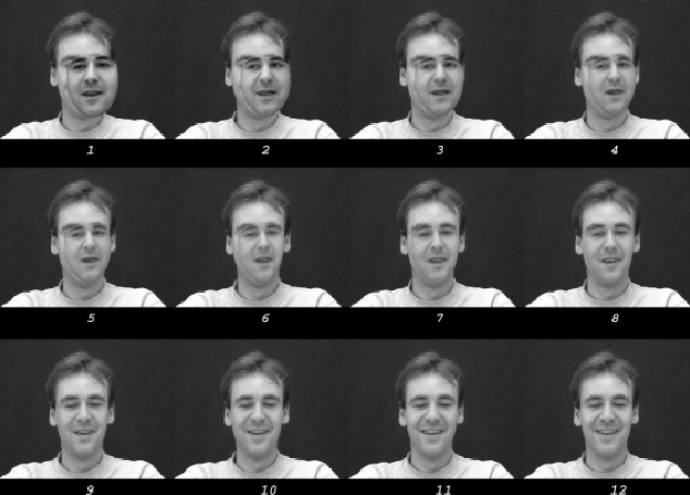
Figure 3.7: Active appearance model search algorithm.

Figure 3.8: Example of application of the active appearance model search algorithm. The figures represent the synthesis of the parameters found after each step of the algorithm.

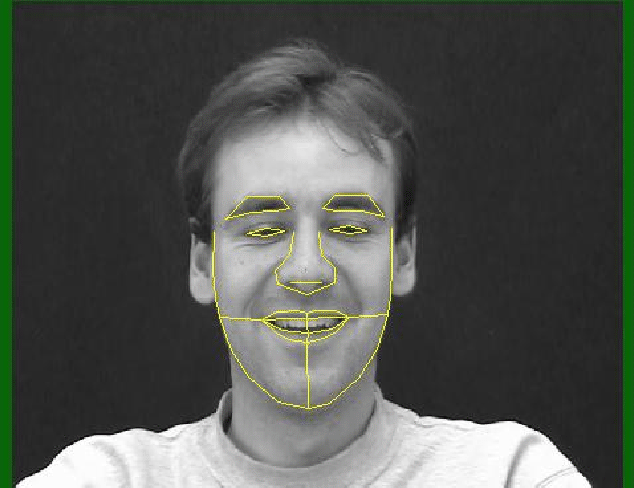
Figure 3.9: Example of result of the AAM search algorithm. The figure represent the synthesis of the shape found overlaid on the original image given to the algorithm. The different appearance parameters found at each steps are synthesised on figure 3.8.