Statistical models of appearance

The aim of the statistical model of appearance is to add information about the texture of an object to the information about the shape of the object. The approach is the same as the statistical shape models. The model is learnt from a set of annotated images of the object.

First, a statistical shape model is built from the training set. New shapes ${\bf x}$ can be generated by the equation:

$${\bf x}=\overline{\bf x}+\Phi_s {\bf b}_s$$ (8)

where ${\bf b}_s$ is a vector of shape parameters.

Then, given the mean shape we warp the training images into a shape-free patch of texture. Figure 3.4 shows how a face is decompose into a shape and a shape-free texture.

Figure 3.4: Decomposition of a face into a shape and a shape-free texture.

The set of shape-free textures is then normalised in order to reduce the effect of lighting. The pixel values are changed by a linear function so that the shape-free texture of a image is as close as possible to the shape-free texture of the normalised mean.

A principle component analysis is then applied to the shape-free texture in order to model this patch by a linear equation:

$${\bf g}=\overline{\bf g}+\Phi_g {\bf b}_g$$ (9)

where ${\bf b}_g$ represents the parameters, as it was already the case with the statistical shape model and $\bf g$ is a vector containing the pixel values of the shape-free texture patch.

${\bf b}_s$ and ${\bf b}_g$ can then describe an object and its texture. Nevertheless, the two vectors can still be correlated. In order to reduce the dimensionality again, we compute the vector:

$${\bf b}=\left(\begin{array}{l} {\bf W}_s{\bf b}_s \\ {\bf b}_g \\ \end{array}\right)$$ (10)

for each training image, where ${\bf W_s}$ is a diagonal matrix of weights that allows to compare ${\bf b_s}$ and ${\bf b_g}$. A third principle component analysis is applied to these data to obtain the model:

$${\bf b}={\bf Q}{\bf c}$$ (11)

where ${\bf c}$ describes the new set of parameters that controls the model. For every ${\bf c}$, an object can be synthesised. This is an important characteristic of the model. It will allow us to synthesise behaviour once the proper parameter stream is found.

The figure 3.5 shows the first mode of variation of such a model.

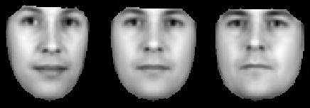
Figure 3.5: Example of the first mode of variation of the face using a statistical model of appearance. The parameter of ${\bf c}$ corresponding to the largest eigenvalue varies from $-3\sqrt{\lambda_1}$ to $3\sqrt{\lambda_1}$.