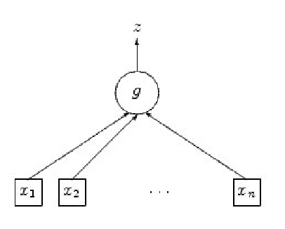
In mathematical terms, a neural network is simply a function with some parameters called weights. This function can be build using a simple element called a neuron. A neuron can be represented by the figure 2.8.
The function ![]() is composed of a linear combination of inputs which is called potential and an activation function
is composed of a linear combination of inputs which is called potential and an activation function ![]() . The potential
. The potential ![]() of a neuron is defined by:
of a neuron is defined by:
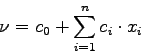
where ![]() is a constant called bias. The bias can be introduced into the sum by introducing a new input of the neuron whose value is always 1. The bias then becomes the parameter associated with this value. So we can write:
is a constant called bias. The bias can be introduced into the sum by introducing a new input of the neuron whose value is always 1. The bias then becomes the parameter associated with this value. So we can write:
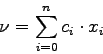
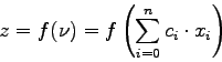
where ![]() . We can then compute the returned value
. We can then compute the returned value ![]() using the formula:
using the formula:
The activation function used is the hyperbolic tangent function or sigmoid. Other sigmoid functions such as
![]() could be used as activation functions.
could be used as activation functions.
These neurons can be combined into a network by providing inputs for neurons using the outputs of other neurons. Such a network is called a neural network. So a neural network can have different number of inputs or outputs, and different architectures.
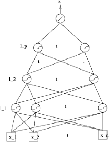
We are particularly interested in an architecture called the multi-layer Perceptron, which figure 2.9 shows. It is composed of ![]() layers,
layers, ![]() to
to ![]() . Each layer is fully connected to the next layer. The output layer has a linear activation function. The other neurons have a sigmoidal activation function.
. Each layer is fully connected to the next layer. The output layer has a linear activation function. The other neurons have a sigmoidal activation function.
 |
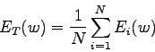
We also need a way to assess the performance of the learned mapping. The evaluation of the error is done using the sum-of-squares error function over a set ![]() . The set
. The set ![]() is a set of pairs. Each pair is composed of an input and the corresponding desired value of the output (target) of the neural network. The sum-of-square function is:
is a set of pairs. Each pair is composed of an input and the corresponding desired value of the output (target) of the neural network. The sum-of-square function is:
This error function has to be minimized with respect to ![]() according to a learning set. The result of this minimization gives us a set of weights which form a trained network. For each regular function, we can find a neural network that can fit this function with an arbitrary precision.
according to a learning set. The result of this minimization gives us a set of weights which form a trained network. For each regular function, we can find a neural network that can fit this function with an arbitrary precision.
We can assess the performance of the training using a test set which is different from the learning set. The computation of the sum-of-square error over this test set gives us a measure of the performance of the neural network.