Experimental procedure

All the previous experiments in the corridor were using a single frame to control the robot. When dealing with odometry, a single frame is not sufficient. We have to use two frames and compute the distance between the two corresponding locations in the room. All the experiments described in this chapter were done in the robotics laboratory with boxes, tables and computers around.

The idea of automatic learning was applied once more. In the beginning, the robot took a picture of the room. Then it moved forward for a random amount of distance and took a second picture of the room. The distance between the two locations was recorded with the internal odometry system. The robot then moved for a random amount of distance again, took a picture, etc.

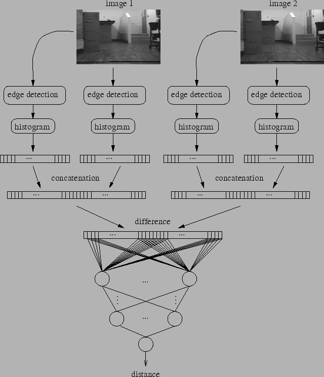
Figure 4.1 shows the processus which was used to preprocess the two different pictures. Each picture was preprocessed by the Difference of Gaussian edge detector in order to extract both vertical and horizontal histograms. The histograms were then concatenated. This gives us two vectors, one per original picture. A possible solution is to concatenate these two vectors to form the input vector used by the multi-layer Perceptron. But there is no reason to give bigger importance to one picture compared to the other. Indeed, if we swap the two pictures, we should end up with the opposite value. So if we concatenate the two vectors, the learned weights corresponding to each vector should be of opposite values or at least, equivalent. Therefore, it makes sense to subtract the two vectors. The resulting vector will be the input of the multi-layer Perceptron.

Figure 4.1: Processus used to extract a distance from two images. The concatenation of vertical and horizontal histograms is computed for each image. The difference of the two resulting vectors is the input of a multi-layer Perceptron.

The neural network used this time is an off-line multi-layer Perceptron. This means that we have to store each pair of training values composed by a vector and a distance measured by the internal odometry. In consequence, the training of the neural network is done after the data acquisition. It is possible to train the neural network on another machine. As the robot hosts a very slow 486 PC, we did the training on another computer: a Pentium $^{\tiny\textcircled{r}}$ III, 500 MHz. Even on such a machine the computation is slow, so a small number of inputs was used due to big stripes. In the experiments, the width of the stripes was 20 pixels for both horizontal and vertical histograms.

Some experiments were done using a uniform probability ${\cal U}\left([0,100]\right)$ from which random travelled distances were extracted. The distances were chosen between $0$ and $10$ inches. Other experiments were using a gaussian distribution ${\cal N}\left(50,20\right)$. The distances were chosen with a average of $5$ inches and a standard deviation of $2$ inches, in order to test the algorithm and to see how it performed on a restricted window only. The algorithms which computed such distributions were taken from [11].