Experimental results

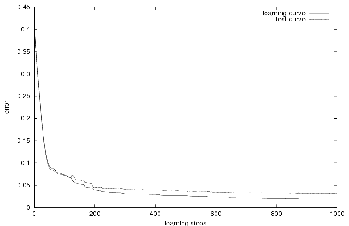
Figure 4.2 shows that the multi-layer Perceptron was able to map a relationship between the pairs in the learning set, that is, between vectors which represents preprocessed images and distances. Indeed, the error computed using a test set decreased during the minimization, so the multi-layer Perceptron performs better and better during the minimization. The parameters used for this learning can be found in table 4.1.

**Figure 4.2:** Egomotion learning curve. The graph shows the error of prediction of a multi-layer Perceptron the weights of which correspond to each points found by the minimization algorithm. Errors made on the learning set and a test set are plotted for each steps.
$\begin{figure}\begin{center}\epsfysize =5cm \epsfbox{ps1comp80l.ps} \end{center} \end{figure}$

**Table 4.1:** Parameters used for the learning of egomotion
multi-layer Perceptron:
number of layers	4
number of neurons in the input layer	53
number of neurons in layer 2	25
number of neurons in layer 3	10
number of neurons in output layer	1
Gradient descent:
number of iterations	60
value of $\eta$	0.01
Quasi-Newton minimization:
number of iterations	940
value of $\tau$	$10^{-4}$
value of	0.3

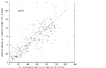
The ideal result of the mapping of the multi-layer Perceptron is the correct distance for each test point. In order to assess our result, we want to see how far away we are from the ideal mapping by studying the correlation between the real output (measures from the odometry) and the computed output (estimations from the multi-layer Perceptron). As the relationship should be linear, we have to compute the correlation coefficient between the real and the computed outputs for each test. Figure 4.3 shows the correlation between estimated and real distances that we computed from a testing set. The linear correlation coefficient is

. This coefficient shows that a relationship exists between the real and the estimated output, but this relationship is not perfect.

**Figure 4.3:** Correlation using an uniform distribution. The graph shows the correlation between the real distances given by the odometry system and the computed distances given by the multi-layer Perceptron.
$\begin{figure}\begin{center}\epsfysize =5cm \epsfbox{ps1comp80rho.ps} \end{center} \end{figure}$

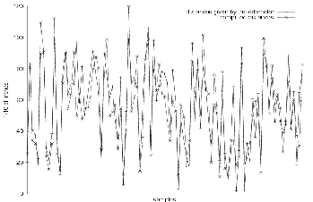
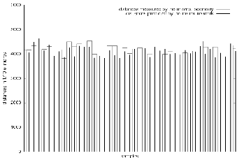
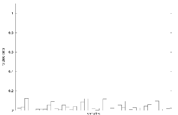
We can also judge the results by plotting the real and the estimated distances for each sample. This is done in figure 4.4. We can also plot the relative error for each sample. Figure 4.5 shows the relative error of the samples corresponding to the samples shown in figure 4.4.

**Figure 4.4:** Differences between the real and the computed distances. For each sample, the graph shows the real distance given by the odometry system and the estimated distance given by the multi-layer Perceptron.
$\begin{figure}\begin{center}\epsfysize =5cm \epsfbox{ps1comp80.ps} \end{center} \end{figure}$

**Figure 4.5:** Relative errors between the real and the computed distances. Note that the big values of the relative errors correspond to the small travelled distances in figure 4.4.
$\begin{figure}\begin{center}\epsfysize =5cm \epsfbox{ps1comp80rerr.ps} \end{center} \end{figure}$

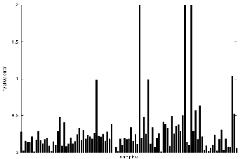The mean of the relative errors of random distances taken from an uniform distribution is approximately 0.4, and the standard deviation is greater than 10. Consequently, the standard deviation suggests that the result cannot be trusted. However, we can note that this bad standard deviation is due to some extreme values which look more like isolated cases than general cases. In fact we can see that these isolated cases correspond to test samples with a small distance measured by the odometry system. Ignoring these particular cases, the results are better. Indeed, the mean and the standard deviation will be smaller. Of course, the mean will not plummet too much, but we cannot expect the relative error to be below 10 % which is the accuracy of the odometry system used to teach the robot how to estimate distances.

An idea that was worth trying is to eliminate small distances during the tests by using a normal distribution centered on the same mean that the original uniform distribution used. This change gives us a windowed testing. Figures 4.6(a), 4.6(b) and 4.6(c) show that the results are not improved with this distribution. The correlation coefficient is now

instead of

above. So the idea of windowed testing does not bring any better results.

**Figure 4.6:** Results using a normal distribution. Big values of the relative error still correspond to the small values of the real corresponding distance. The results are not better than above.
$\begin{figure}\begin{center} \subfigure[Correlation]{\epsfysize =5cm \epsfbox{... ...errors]{\epsfysize =5cm \epsfbox{ps1comp81rerr.ps} } \end{center} \end{figure}$

However, robots are usually required to navigate for a long time and therefore they travel a long distance. So when we want to design a navigation system, we do not really want to worry about small distances. Long distances are definitely more interesting because the internal odometry of a robot makes bigger mistakes after a long distance than after a small distance. Indeed, errors done are often cumulative because of the nature of the contact between the robot and the ground. Furthermore, the friction coefficient between the robot and the ground changes according to the location. For instance, the friction coefficient was not the same in the laboratory and in the corridors.

In these two cases, visual odometry can be more powerful than the internal odometry of the robot based on wheel encoders. Indeed, visual odometry uses global landmarks. So the accuracy of the measures is the same everywhere and the error is often centered around zero. This was the case for the aforementioned experiments, as we can see on figure 4.7.

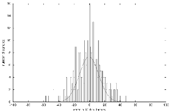**Figure 4.7:** Distribution of the error during the tests. The error done by the multi-layer Perceptron seems to follow a gaussian distribution centered around zero.
$\begin{figure}\begin{center}\epsfysize =5cm \epsfbox{ps1comp81gauss.ps} \end{center} \end{figure}$

As we can see, the error function can be modeled by a gaussian centered around zero. Besides, we know that a sum of gaussian distributions, sharing the same mean and standard deviation, is stable by addition. In particular if the mean of those distribution is zero, then the mean of the sum of those very

distributions remains zero and the standard deviation is $\sqrt{n}$ times the standard deviation of any one of the gaussian distributions contributing in the sum. For instance, if we take 80 distances that come all from a gaussian distribution ${\cal N}(0,15)$ the sum of all those distances comes from a gaussian distribution ${\cal N}\left(0,15\sqrt{80}\right)$ .

The estimation of a longer distance was computed using path integration. Consecutive distance estimations were done and added. The resulting estimation of the total travelled distance is shown on figure 4.8. The total travelled distance during the experiments was approximately $10\;m$ . Figure 4.9 shows that the corresponding relative error is less than the previous relative errors. The result is even better than expected. We have a mean of $3.9\%$ of relative error with a standard deviation of $3.3\%$ . So the distance measured by the multi-layer Perceptron is better than the distance given by the odometry in more than $90\%$ of cases. This confirms that visual odometry is better than internal odometry based on wheels for long distances.

**Figure 4.8:** Estimation of a long distance. The graph shows the real distances travelled measured by the odometry and the distances estimated by the multi-layer Perceptron.
$\begin{figure}\begin{center}\epsfysize =5cm \epsfbox{psfinalest.ps} \end{center} \end{figure}$

**Figure 4.9:** Relative error during a long distance. The relative error is less than in more than $90\%$ of cases.
$\begin{figure}\begin{center}\epsfysize =5cm \epsfbox{ps1finalrerr.ps} \end{center} \end{figure}$