Appearance model based methods

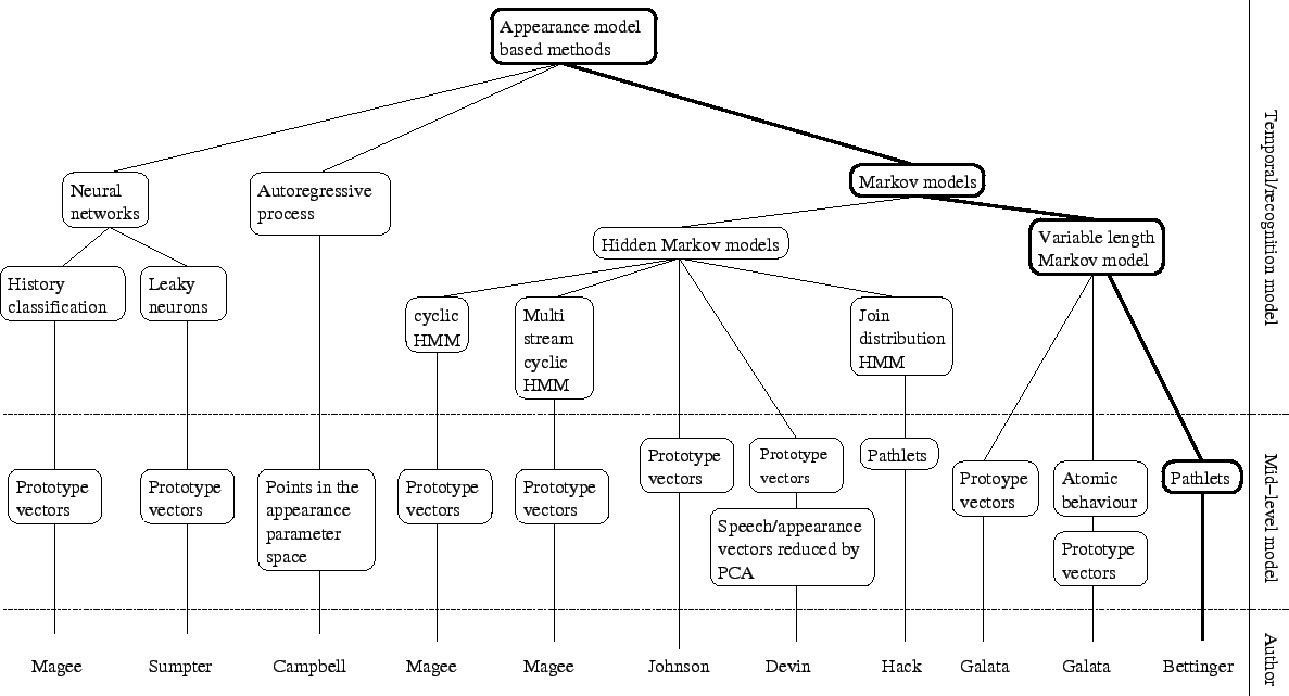
Figure 2.5 summarises some of the techniques using appearance models. Such models represent the shape and texture of an object (see section 3.4), and have been found to be very effective for synthesising faces and facial behaviour.

Figure 2.5: Appearance model based methods in behaviour modelling. The branch corresponding to our model is enhanced using bold lines.

Magee and Boyle [62] built a behaviour classifier called ``history space classifier''. The history space is constructed by a succession of a spacial and a temporal operator. The spacial operator selects the nearest prototype using a winner take all approach. The temporal operator used is simply a multiplication by a weight which is the reciprocal of the time spent since the prototype has last been selected [60]. A more complex temporal operator could be used such as a set of leaky neurons as has been done by Sumpter and Bulpitt [92]. A modified version of the expectation maximisation introduced by Cootes and Taylor [23] is then used to model the point distribution function. In order to decrease the computational load of the algorithm, a principle component analysis is applied before the expectation maximisation algorithm so that the size of the data set is reduced. The resulting point distribution function is then used to predict the next state in the sequence.

Magee and Boyle [61] are using cyclic hidden Markov models in order in conjunction with Black and Jepson's variant of the particle filtering algorithm. Their aim is to recognise cows having difficulty walking. Figure 2.8(d) shows how hidden nodes are connected in a cyclic hidden Markov model. Those models are good at describing the cyclic motion that can be observed from a cow's leg. Two cyclic hidden Markov models are used to model the motion of cows walking. One learns a typical behaviour of a healthy cow and the other one learns a lame behaviour. The cyclic hidden Markov models are integrated in the re-sampling particle filtering framework so that the model that described a test behaviour more accurately dominates over time. The decision is then based on the number of samples produced for each model. In [61], Magee et al. also use a multi-stream cyclic hidden Markov model to model the two motions with only one stream of hidden states.

In [51], shapes are approximated by splines. The parameters controlling the splines as well as their speed are first clustered into prototype vectors using a competitive learning neural network. A compressed sequence derived from the prototype vector sequence is learnt using a Markov chain. A cubic Hermite interpolation is used along with the learnt Markov chain to recover the temporal structure of the sequence before compression and to extrapolate a behaviour. Furthermore, for generation purposes, a single hypothesis propagation and a maximum likelihood framework are described. During the generation, states of the Markov chain are chosen according to the state of the shape of a tracked person. This can allow generation of a shape of a virtual partner driven by a tracked real person. In [28], Devin and Hogg added sound and appearance to the framework in order to demonstrate that producing a talking head is possible.

Galata, Johnson and Hogg [33] also split trajectories into prototypes in order to model movement. The structure of the movements is then learnt using a variable length Markov model. As this approach seems to be one of the state of the art in behaviour modelling, we studied its components, in particular the variable length Markov model (see chapter 6). A prototype clustering is performed using a $k$-means like algorithm. The sequence of prototypes is then learnt using the variable length Markov model. The advantage of this approach is that it can model joint behaviour of people [52]. This is an essential characteristic for building a realistic human-computer interface. In [34], sequences of prototypes delimited by key-frames prototypes form atomic behaviours. The variable length Markov model can learn those atomic behaviours instead of directly learning the prototypes, thus producing a higher level model.

Hack et al. [40] model trajectories by a sequence of pathlets. The dimensions of the pathlets observed in a training sequence are reduced using a principle component analysis. Using a Gaussian hidden Markov model, pairs of consecutive pathlets are clustered. New sequences of pathlets can then be created by sampling pairs of pathlets from the model, constrained by the choice of the first pathlet being the second pathlet of the previous sampled pathlet pair. This assures continuity in the sampling of pathlets through the generated sequence.

Campbell et al. [17] introduce another way of generating video sequences of faces based on an existing video clip without direct reuse of the original frames. They encode frames from the original sequence using an appearance model and a trajectory is obtained in the parameter space. This trajectory is then learnt using a second order autoregressive process. An autoregressive process predicts the position of a point ${\bf y_k}$ in the appearance parameter space, given the two previous points ${\bf y_{k-1}}$ and ${\bf y_{k-2}}$ where ${\bf k}$ represents the frame number, using the equation:

$${\bf y_k}-{\bf\overline{y}}={\bf A_2}\left({\bf y_{k-2}}-{\b... ...eft({\bf y_{k-1}}-{\bf\overline{y}}\right)+{\bf B_0} {\bf w_k}$$ (1)

where ${\bf\overline{y}}$ is the limit of the mean value of ${\bf y_k}$ as ${\bf k}$ tends to infinity, ${\bf w_k}$ contains white noise ( ${\bf w_k} \sim {\cal{N}} \left(0,1\right)$), ${\bf A_2}$, ${\bf A_1}$ and ${\bf B_0}$ are parameter matrices. ${\bf\overline{y}}$, ${\bf A_2}$, ${\bf A_1}$ and ${\bf B_0}$ are learnt from the original data set. The learning method used in this work is due to Reynard et al. and is described in [79]. Given two initial points in the parameter space, a new trajectory can be generated by applying equation 2.1 repetitively. This new trajectory can be used to synthesise a video sequence of a face. They use this model in [74] and [38] to create an expression space that can be easily displayed and to help animators to generate new video sequences of expressions from an intuitive interface.